SEDs

We provide a large grid of CLUMPY model spectral energy distributions (SED) in the form of an hdf5 file:

Download:	clumpy_models_201410_tvavg.hdf5 (1.2 GB) (md5sum: 4641c5def6bcc1ee63f0e13184d056ca)

hdf5 is a hierarchical and versatile data format, allowing to store all kinds of datasets in the same file. Below you can find a brief explanation of the stored content, and a few examples how to access the models with Python.

Datasets

Inspect the content of the HDF5 file (here with Python, and the h5py module installed):

import h5py

h = h5py.File('clumpy_models_201410_tvavg.hdf5')

# see what's there
h.items()

[(u'N0', <HDF5 dataset "N0": shape (1247400,), type "<i4">),
(u'Y', <HDF5 dataset "Y": shape (1247400,), type "<i4">),
(u'f2', <HDF5 dataset "f2": shape (1247400,), type "<f4">),
(u'flux_tor', <HDF5 dataset "flux_tor": shape (1247400, 119), type "<f4">),
(u'flux_toragn', <HDF5 dataset "flux_toragn": shape (1247400, 119), type "<f4">),
(u'i', <HDF5 dataset "i": shape (1247400,), type "<i4">),
(u'lam10', <HDF5 dataset "lam10": shape (1247400,), type "<f8">),
(u'lam18', <HDF5 dataset "lam18": shape (1247400,), type "<f8">),
(u'ptype1', <HDF5 dataset "ptype1": shape (1247400,), type "<f4">),
(u'q', <HDF5 dataset "q": shape (1247400,), type "<f4">),
(u's10', <HDF5 dataset "s10": shape (1247400,), type "<f4">),
(u's18', <HDF5 dataset "s18": shape (1247400,), type "<f4">),
(u'sig', <HDF5 dataset "sig": shape (1247400,), type "<i4">),
(u'tv', <HDF5 dataset "tv": shape (1247400,), type "<f4">),
(u'wave', <HDF5 dataset "wave": shape (119,), type "<f8">)]

As you can see there are 1,247,400 models in the database, with 119 wavelength per SED. The CLUMPY parameters are \(N_0,Y,i,q,\sigma,\tau_V\), or here N0,Y,i,q,sig,tv. The wavelength array is wave. Some derived properties are also stored: f2 (dust covering fraction), ptype1 (the probability to see the AGN unobscured), s10 & s18 (the 10 & 18-micron silicate feature strengths), lam10 & lam18 (the wavelengths where the extrema of the 10 and 18-micron features occur). Finally, the model SEDs are stored in flux_tor (torus-only SED) and flux_toragn (torus with AGN input spectrum added in, regardless of the actual probability to see the AGN in that model). The spectral shapes are \(\lambda\,F_\lambda\) (in relative units), and the wavelength are in mircon.

Sampled parameter values

Print the sampling of all free model parameter values (except wavelength):

params = ('N0','Y','q','sig','tv','i')
for par in params:
    print "%4s  %s" % (par,', '.join([str(e) for e in N.unique(h[par][:])]))

 N0  1, 2, 3, 4, 5, 6, 7, 8, 9, 10, 11, 12, 13, 14, 15
  Y  5, 10, 20, 30, 40, 50, 60, 70, 80, 90, 100
  q  0.0, 0.5, 1.0, 1.5, 2.0, 2.5, 3.0
sig  15, 20, 25, 30, 35, 40, 45, 50, 55, 60, 65, 70
 tv  10.0, 20.0, 40.0, 60.0, 80.0, 120.0, 160.0, 200.0, 300.0
  i  0, 10, 20, 30, 40, 50, 60, 70, 80, 90

Accessing the SEDs

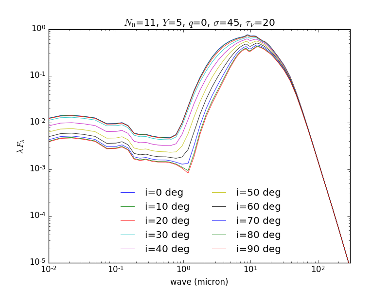
Accessing the data is as trivial as working with arrays in Python. Here we plot a few SEDs:

import pylab as p

wave = h['wave'][:]  # load wave array

# load SEDs
start = 63010   # some random index
n = 10          # get 10 models in total
seds = h['flux_tor'][start:start+n,:]  # load 10 SEDs, all wavelengths

# plot
for j in xrange(n):
    p.loglog(wave,seds[j,:],ls='-',lw=0.8,alpha=0.8,label='i=%d deg'%h['i'][start+j])

p.xlabel('wave (micron)')
p.ylabel(r'$\lambda\,F_\lambda$')
p.xlim(1e-2,300)
p.ylim(1e-5,1)
title = r"$N_0$=%g, $Y$=%g, $q$=%g, $\sigma$=%g, $\tau_V$=%g" %\
          tuple([h[par][start] for par in ('N0','Y','q','sig','tv')])
p.title(title)
p.legend(loc='lower center',frameon=False,ncol=2)
p.savefig('seds.png',dpi=100)

Accessing other datasets

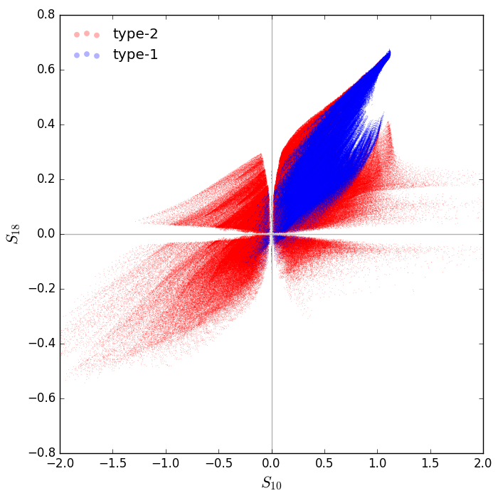
Now let's plot the 10 and 18 micron silicate feature strengths of all SEDs, for separately for type-1 and type-2 models:

# load some parameter arrays into RAM
ptype1 = h['ptype1'][:]
s10 = h['s10'][:]
s18 = h['s18'][:]

# make selection mask for all type1 models
type1 = (ptype1 > 0.5)  # probablity to see the AGN > 50%

# plot an s10 vs. s18 diagram
fig = p.figure(figsize=(7,7))
p.scatter(s10[~type1],s18[~type1],marker='.',s=2,linewidths=0,c='r',alpha=0.3,edgecolors='none',label='type-2')
p.scatter(s10[type1],s18[type1],marker='.',s=2,linewidths=0,c='b',alpha=0.3,edgecolors='none',label='type-1')
p.xlim(-2,2)
p.ylim(-0.8,0.8)
p.axvline(0,c='0.7')
p.axhline(0,c='0.7')
p.xlabel(r'$S_{10}$',fontsize=16)
p.ylabel(r'$S_{18}$',fontsize=16)
p.legend(loc='upper left',frameon=False,markerscale=8)
fig.subplots_adjust(left=0.12,right=0.97,top=0.97,bottom=0.09)
p.savefig('s10s18.png',dpi=100)